
Disclaimer: this lesson was adapted from an old tutorial done in collaboration with Francesco Pelosin.
In this lesson, you will learn how to efficiently use NumPy one of the most well-known packages for scientific programming in Python.
A package ($\approx$ library) is a collection of code scripts
(called modules) with a specific purpose. Whenever you want to use the
features in a package, you must import the package first with the import
keyword. You can give a shorter alias to the package name with the as
keyword.
import numpy as np
ndarray
NumPy’s core data structure is the ndarray, that is, a multidimensional
array, corresponding to a mathematical tensor:
ndarray1D → vector$$\begin{pmatrix} 1 & 5 & 7 & 2 \end{pmatrix}$$
ndarray2D → matrix$$\begin{pmatrix} 1 & 5 & 7 & 2 \\ 4 & 3 & 2 & 0 \\ 3 & 6 & 1 & 8 \end{pmatrix}$$
ndarray3D → tensor 3D …ndarray4D → tensor 4D ……
You can think of a ndarray as a Python list with mathematical superpowers.
Let’s build our first ndarray, containing three values. In order to do this I
have to pass a list of three numbers to the np.array function.
a = np.array([0, 1, 2])
A ndarray is characterized by two important metadata:
shape→ the dimensions of thendarraydtype→ the type of the elements stored in thendarray(decimal, integer, etc.)
print(f'a shape: {a.shape}')
print(f'a dtype: {a.dtype}')
a shape: (3,)
a dtype: int64
(3,) means that the array has only one dimension, with three values.
int64 means that the data contain integer values, and each value is stored in
the memory in a binary format that requires 64 bits.
Let’s instantiate now a 2D ndarray of size $3 \times 3$ containing integer
numbers. For two dimensions, the trick consists of using a list of lists.
b = np.array([[0, 1, 2],
              [3, 4, 5],
              [6, 7, 8]])
b
array([[0, 1, 2],
       [3, 4, 5],
       [6, 7, 8]])
print(f'b shape: {b.shape}')
print(f'b dtype: {b.dtype}')
b shape: (3, 3)
b dtype: int64
Let’s build now an ndarray with shape (3, 2, 2)
c = np.array([[[1,2], [3,4]], [[5,6], [7,8]], [[9,10], [11,12]]])
print(c)
print(c.shape)
[[[ 1  2]
  [ 3  4]]

 [[ 5  6]
  [ 7  8]]

 [[ 9 10]
  [11 12]]]
(3, 2, 2)
An ndarray with shape (n,) behaves like one with shape (1, n) but it
is different from one with shape (n,1). In mathematical terms, they
correspond to vectors $u \in \mathbb{R}^n$, $v \in \mathbb{R}^{1 \times n}$ and
$w \in \mathbb{R}^{n \times 1}$
u = np.random.rand(3)
v = np.random.rand(1, 3)
w = np.random.rand(3, 1)
print(f'u: {u}, of shape {u.shape}')
print(f'v: {v}, of shape {v.shape}')
print(f'w: {w}, of shape {w.shape}')
u: [0.8411285  0.86529657 0.8823971 ], of shape (3,)
v: [[0.24990387 0.99244299 0.91256392]], of shape (1, 3)
w: [[0.99928425]
    [0.20520275]
    [0.82996469]], of shape (3, 1)
Create a ndarray
In the previous example we have used a new function, np.random.rand, that has
generated values that have not been explicitly written.
Writing by hand all values of an ndarray might be a very long task, if not
impossible. For this reason, there exist some useful functions to create
standard ndarrays.
np.zeros(shape): ndarray with only 0.
z = np.zeros((3, 3, 3))
z
array([[[0., 0., 0.],
        [0., 0., 0.],
        [0., 0., 0.]],

       [[0., 0., 0.],
        [0., 0., 0.],
        [0., 0., 0.]],

       [[0., 0., 0.],
        [0., 0., 0.],
        [0., 0., 0.]]])
np.ones(shape): ndarray with only 1.
o = np.ones((5,))
o
array([1., 1., 1., 1., 1.])
np.full(shape, fill_value): ndarray initialized with the same values
specified by fill_value
f = np.full((4, 3), fill_value=3.14)
f
array([[3.14, 3.14, 3.14],
       [3.14, 3.14, 3.14],
       [3.14, 3.14, 3.14],
       [3.14, 3.14, 3.14]])
np.empty(shape): ndarray with uninitialized values. The values displayed
are called dirty. The have been computed by some other previous operations,
they are not needed anymore, and they were left in the memory.
e = np.empty((3, 4))
e
array([[3.14, 3.14, 3.14, 3.14],
       [3.14, 3.14, 3.14, 3.14],
       [3.14, 3.14, 3.14, 3.14]])
np.random.rand(shape): ndarray with random values from 0 (included) to 1
(excluded).
rnd = np.random.rand(2, 3)  # no tuple needed here!
rnd
a = 2
b = 5
a + (b - a) * np.random.rand(2, 3)
array([[3.7885215 , 4.87429192, 4.17208196],
       [3.54320931, 2.39380702, 3.42507703]])
np.arange(low, high): ndarray with a sequence of integers between low
(included) e high (excluded)
rng = np.arange(9)  # dtype = integer
print(rng)
frng = np.arange(1., 10.)  # dtype = float
print(frng)
[0 1 2 3 4 5 6 7 8]
[1. 2. 3. 4. 5. 6. 7. 8. 9.]
Operations on ndarrays
In the following, we revise some more advanced operations that manipulate arrays to get new ones.
Change shape
the shape of a ndarray can be modified through ndarray.reshape(shape)
rng = rng.reshape(3, 3)
print(rng.shape)
print(rng)
(3, 3)
[[0 1 2]
 [3 4 5]
 [6 7 8]]
f = f.reshape(2, 2, -1)  # infer dimension 2: (12 / (2 * 2)) = 3
print(f.shape)
print(f)
(2, 2, 3)
[[[3.14 3.14 3.14]
  [3.14 3.14 3.14]]

 [[3.14 3.14 3.14]
  [3.14 3.14 3.14]]]
To “stretch out” a ndarray we can use the functions ndarray.flatten or
ndarray.ravel, obtaining a 1D ndarray with shape (n,). The only
difference between the two functions is that flatten creates a new ndarray
while ravel not.
rnd1 = rnd.flatten()
rnd2 = rnd.ravel()

rnd1[0] = 0.
print(f'rnd1: {rnd1}')
print(f'rnd: {rnd}')

print()

rnd2[0] = 1.
print(f'rnd2: {rnd2}')
print(f'rnd: {rnd}')
rnd1: [0.         0.18214381 0.55497825 0.00390567 0.12822584 0.23463752]
rnd: [[0.79350509 0.18214381 0.55497825]
 [0.00390567 0.12822584 0.23463752]]

rnd2: [1.         0.18214381 0.55497825 0.00390567 0.12822584 0.23463752]
rnd: [[1.         0.18214381 0.55497825]
 [0.00390567 0.12822584 0.23463752]]
Let’s try now some simple operations with ndarrays.
Sum
$$ \begin{pmatrix} 3 & 2 & 4 \\ 5 & 1 & 10 \\ 7 & 2 & 9 \end{pmatrix} + \begin{pmatrix} 1 & 4 & 7 \\ 12 & 5 & 0 \\ 3 & 2 & 1 \\ \end{pmatrix} = \begin{pmatrix} 4 & 6 & 11 \\ 17 & 6 & 10 \\ 10 & 4 & 10 \\ \end{pmatrix} $$
x = np.array([[3., 2., 4.], [5., 1., 10.], [7., 2., 9.]])
y = np.array([[1., 4., 7.], [12., 5., 0.], [3., 2., 1.]])
print(x + y)
[[ 4.  6. 11.]
 [17.  6. 10.]
 [10.  4. 10.]]
Scalar-vector product
$$ 3 \cdot \begin{pmatrix} 3 & 2 & 4 \\ 5 & 1 & 10 \\ 7 & 2 & 9 \end{pmatrix} = \begin{pmatrix} 9 & 6 & 12 \\ 15 & 3 & 30 \\ 21 & 6 & 27 \end{pmatrix} $$
k = 3
print(k * x)
[[ 9.  6. 12.]
 [15.  3. 30.]
 [21.  6. 27.]]
Hadamard Product
$$ \begin{pmatrix} 3 & 2 & 4 \\ 5 & 1 & 10 \\ 7 & 2 & 9 \end{pmatrix} \odot \begin{pmatrix} 1 & 4 & 7 \\ 12 & 5 & 0 \\ 3 & 2 & 1 \\ \end{pmatrix} = \begin{pmatrix} 3 & 8 & 28 \\ 60 & 5 & 0 \\ 21 & 4 & 9 \\ \end{pmatrix} $$
print(x * y)
[[ 3.,  8., 28.],
 [60.,  5.,  0.],
 [21.,  4.,  9.]]
Matrix Product
$$ \begin{pmatrix} 3 & 2 & 4 \\ 5 & 1 & 10 \\ 7 & 2 & 9 \end{pmatrix} \times \begin{pmatrix} 1 & 4 & 7 \\ 12 & 5 & 0 \\ 3 & 2 & 1 \\ \end{pmatrix} = \begin{pmatrix} 39 & 30 & 25 \\ 47 & 45 & 45 \\ 58 & 56 & 58 \\ \end{pmatrix} $$
print(x @ y) # or np.dot(x, y)
[[39., 30., 25.],
 [47., 45., 45.],
 [58., 56., 58.]]
Scalar + matrix
z = np.zeros((3,3))
z + 2
array([[2., 2., 2.],
       [2., 2., 2.],
       [2., 2., 2.]])
Scalar $\times$ matrix
z = np.ones((3,3))
z * 2
array([[2., 2., 2.],
       [2., 2., 2.],
       [2., 2., 2.]])
powers, exp, sin, cos, log, etc.
print(x ** 2)  # squares of x
print(np.exp(x))
print(np.sin(y))
[[  9.   4.  16.]
 [ 25.   1. 100.]
 [ 49.   4.  81.]]
[[2.00855369e+01 7.38905610e+00 5.45981500e+01]
 [1.48413159e+02 2.71828183e+00 2.20264658e+04]
 [1.09663316e+03 7.38905610e+00 8.10308393e+03]]
[[ 0.84147098 -0.7568025   0.6569866 ]
 [-0.53657292 -0.95892427  0.        ]
 [ 0.14112001  0.90929743  0.84147098]]
Aggregation functions
We can also perform some aggregation function on an ndarray, such as the sum
or the mean.
print(x.sum())  # sum all values
print(y.mean())  # compute the mean of all values
print(x.min(), x.max())
43.0
3.888888888888889
1.0 10.0
And we can specify that the aggregations be performed only over a specified
dimension, using the axis parameter.
print(x.sum(axis=0))  # compute the sum of each column
print(y.mean(axis=1)) # compute the mean of each row
[15.  5. 23.]
[4.         5.66666667 2.        ]
ndarray indexing
Sometimes it is necessary to access a subset of the values in a ndarray. This
operation is called indexing. Following, some examples. Note that rows and
columns starts from the index 0:
$$ m = \begin{pmatrix} 0 & 1 & 2 \\ 3 & 4 & 5 \\ 6 & 7 & 8 \\ 9 & 10 & 11 \\ 12 & 13 & 14 \end{pmatrix}$$
m = np.arange(15.).reshape(5, 3)
m
array([[ 0.,  1.,  2.],
       [ 3.,  4.,  5.],
       [ 6.,  7.,  8.],
       [ 9., 10., 11.],
       [12., 13., 14.]])
$m_{12} = \begin{pmatrix} 5 \end{pmatrix}$
print(m[1, 2])
print(m[0,0])
5.0
0.0
$$m_{1*} = \begin{pmatrix} 3 & 4 & 5 \end{pmatrix}$$
m[1, :]
m[:, 1]
array([ 1., 4., 7., 10., 13.])
$$m_{1:6, *} = \begin{pmatrix}
3 & 4 & 5 \\
6 & 7 & 8 \\
9 & 10 & 11 \\
12 & 13 & 14
\end{pmatrix}$$
N.B. If the interval exceeds the number of rows/columns of the matrix, NumPy
returns still the maximum possible number of rows/columns. For example, the
row indices in $m$ are from $0$ to $4$. Using 1:6, the rows from $1$
to $4$ are selected.
m[1:6, :]
array([[ 3.,  4.,  5.],
       [ 6.,  7.,  8.],
       [ 9., 10., 11.],
       [12., 13., 14.]])
$$m_{1:5, 2:} = \begin{pmatrix} 5 \\ 8 \\ 11 \\ 14 \end{pmatrix}$$
m[1:5, 2:]
array([[ 5.],
       [ 8.],
       [11.],
       [14.]])
$$\begin{pmatrix} m_{10} & m_{12} & m_{31} \end{pmatrix} = \begin{pmatrix} 3 & 5 & 10 \end{pmatrix}$$
N.B In this case the returned ndarray has always shape (n,)
m[[1, 1, 3], [0, 2, 1]]
array([ 3., 5., 10.])
With the boolean masks I can select the elements that satisfy a condition,
evaluating to True
$$\begin{pmatrix} m_{00} & m_{12} & m_{20} & m_{21} & m_{30} & m_{31} & m_{32} \end{pmatrix} = \begin{pmatrix} 0 & 5 & 6 & 7 & 9 & 10 & 11 \end{pmatrix}$$
N.B. In this case too the returned ndarray has always shape (n,)
mask = np.array([[True, False, False],
                 [False, False, True],
                 [True, True, False],
                 [True, True, True],
                 [False, False, False]])
m[mask]
array([ 0., 5., 6., 7., 9., 10., 11.])
All elements strictly greater than 5.
m[m > 5] # m > 5 returns a boolean mask, directly used for indexing m
array([ 0., 5., 6., 7., 9., 10., 11.])
For more information check NumPy’s indexing conventions
scipy, matplotlib, scikit-learn
NumPy provides mostly low level functions on arrays and some algebraic operation. Other packages have been developed on top of NumPy for higher-level tasks:
- SciPy: extension of NumPy used for optimization, integration, interpolation, linear algebra and statistics.
- matplotlib: a low-level plotting package. Its use is a bit counterintuitive at first, so a new extension, seaborn, became popular.
- scikit-learn: package containing traditional machine learning algorithms. We will use it in the next lessons.
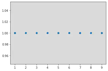
Here is a small example of matplotlib plots, which generates ten dots $(x_i, y)$ with $x_i = i$ (with $i$ ranging from $1$ to $9$) and $y = 1$:
import matplotlib.pyplot as plt

x = np.arange(1, 10)
y = np.ones(9)

plt.scatter(x, y)
plt.show()
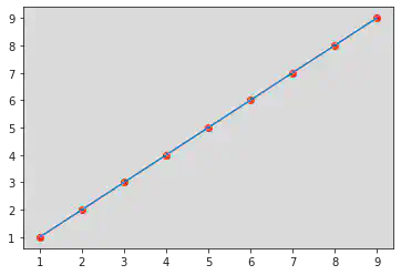
Plotting a line and red points over it:
plt.plot(x, x)
plt.scatter(x, x, c="r")
plt.show()
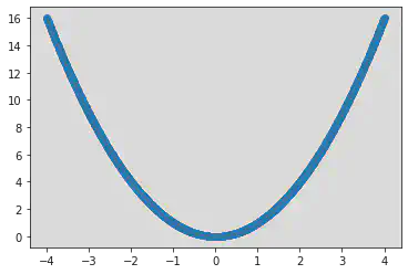
Plotting a parabola using linspace, which produces a ndarray of equispaced
values between a lower and upper bound (this is one of the rare cases where the
upper bound is included).
x = np.linspace(-4, 4, 1000)  # create 1000 points between -4 and 4 (included)
y = x ** 2
plt.plot(x, y)
plt.show()
Exercises (from easy to impossible!)
- Declare an array
arof integers ranging from $1$ to $9$ - Set to $-1$ the elements from index $4$ onward
- Declare an array
ar1of integers ranging from $1$ to $9$ and change its shape to get a $3 \times 3$ matrix - Add $1$ to all values
- Add $1$ to all the values of the second column
- Select and print all the elements in the diagonal of
ar1(Hint: start using Google + NumPy docs) - Set all the elements of the diagonal to $0$
- Plot a series of points from $(1, 1)$ to $(9, 9)$, plot also a line connecting them
- Plot a parabola $y = x^2 + 1$ in the interval $[-4, 5]$. Use
np.linspaceto generate the $x$s - Plot $sin(x)$ and $cos(x)$ with two different colors in the range $x \in [-10, 10]$
- Plot the Ballmer peak with the xkcd theme
If you have arrived here congratulations! You are now proficient in NumPy, here is your graduation cap